First, since our task is to predict the trajectory, according to the properties of recurrent neural networks we need to set up a sliding window to predict one of the later data points based on the previous data. For example, we predict the 11th data point based on the features of the previous 10 data points. Then the 1st through 11th data points are used as inputs to predict the 12th data point, and so on. Here we use the following code to implement it:

def sliding_windows(data, seq_length):
    x = []
    y = []

    for i in range(len(data) - seq_length - 1):
        _x = data[i:(i + seq_length)]
        _y = data[i + seq_length]
        x.append(_x)
        y.append(_y)

    return np.array(x), np.array(y)

seq_length = 30
              

Here we use MSE as the loss function. The parameters are tuned using Adam optimizer. Since these can be implemented directly using the PyTorch framework and are not the focus of this study, their rationale is ignored.

criterion = nn.MSELoss()
optimizer = torch.optim.Adam(gru.parameters(), lr=learning_rate)               
              

In addition, we divide the dataset into a training set and a test set. Among them, the first 90% of the data is the training set to ensure that the model is adequately trained. The last 10% is the test set to test the performance of the dataset.

First, we tried to train the model by feeding three features (latitude, longitude, and altitude) into it and tested its effectiveness. The test results are shown below.

for epoch in range(num_epochs):
    gru.train()
    outputs = gru(trainX)
    optimizer.zero_grad()
    train_loss = criterion(outputs, trainY)
    train_losses.append(train_loss.item())
    train_loss.backward()
    optimizer.step()
    with torch.no_grad():
        gru.eval()
        test_outputs = gru(testX)
        test_loss = criterion(test_outputs, testY)
        test_losses.append(test_loss.item())
    print("Epoch: %d, loss: %1.5f" % (epoch, math.sqrt(train_loss.item())))
              

We can find that both GRU and LSTM perform poorly when predicting three features simultaneously. Therefore, we try other approaches.

First, we try to model the performance of predicting one-dimensional data, tested here using only longitude:

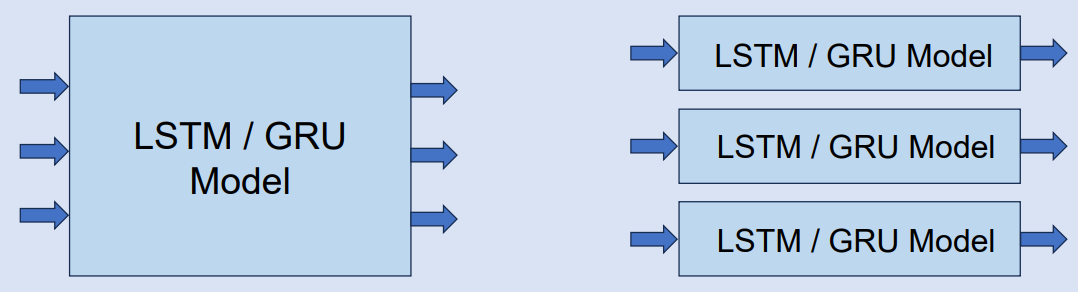
We find that the model is far more effective when it makes single-feature predictions than multi-feature predictions. In the case of GRU, for example, when predicting single data, the loss (RMSE) can be as high as 0.00299. However, when predicting multi-dimensional data, the loss can be as high as 0.01970. This is almost a 6.5 times difference in performance. So we try to use three models to train each of the three data (latitude, longitude and altitude) and then predict each of the three data.

for epoch in range(num_epochs):
    # Training longitude
    gru_long.train()
    outputs_long = gru_long(trainX_long)
    optimizer_long.zero_grad()
    loss_long = criterion(outputs_long, trainY_long)
    train_losses_long.append(loss_long.item())
    loss_long.backward()
    optimizer_long.step()

    # Training latitude
    gru_lat.train()
    outputs_lat = gru_lat(trainX_lat)
    optimizer_lat.zero_grad()
    loss_lat = criterion(outputs_lat, trainY_lat)
    train_losses_lat.append(loss_lat.item())
    loss_lat.backward()
    optimizer_lat.step()

    # Training Altitude
    gru_alt.train()
    outputs_alt = gru_alt(trainX_alt)
    optimizer_alt.zero_grad()
    loss_alt = criterion(outputs_alt, trainY_alt)
    train_losses_alt.append(loss_alt.item())
    loss_alt.backward()
    optimizer_alt.step()

    print("Epoch: %d, Train Loss: %1.5f" % (epoch, math.sqrt(loss_long.item())))
            
              

Therefore, we can try to predict each of these three data using three models as following:

The following is a demonstration of the prediction results:

We can notice much better results than before. Finally, we can generalize this approach to more places for predicting multidimensional data.